Decision Trees

Decision trees are nonparametric statistical models that generate predictions by stratifying a given set of predictors $X$ into a number of simple regions, then predicting the outcome for each of these regions using either the mean (for regression problems) or the mode (for classification problems) of the response variable for all observations contained in that region.

Here’s an example of what a decision tree might look like for a regression problem:

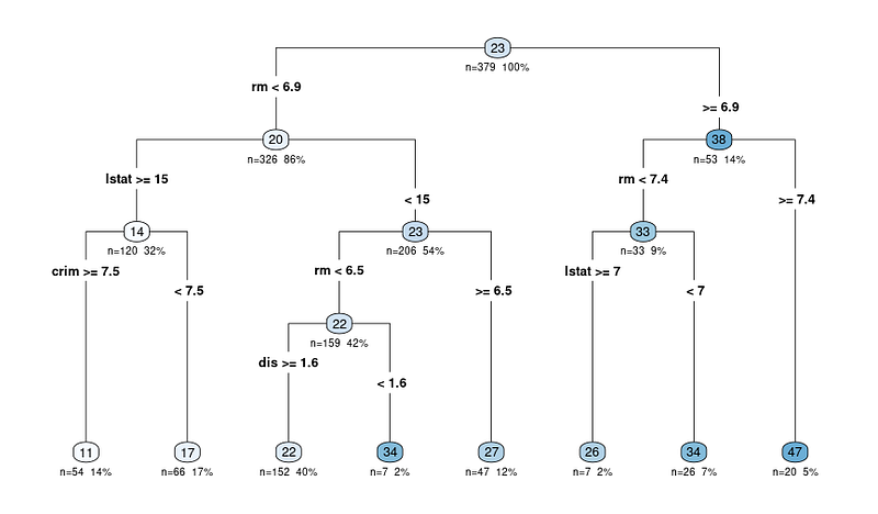
One of the benefits of decision trees is that they’re easy to interpret. They may also more accurately represent human decision processes than something like linear regression.

The biggest drawback of decision trees is that individual trees tend to make pretty poor predictions, largely because they’re high-variance models. Approaches such as random forests or boosting tend to solve this issue, but at the cost of some interpretability.

Building a Regression Tree

Broadly, the steps for building a regression tree are:

1. Split the predictor space, $X$, into $j$ distinct and nonoverlapping regions, $R_1,R_2,...,R_j$
2. For every observation in $R_j$, predict the mean of the $y$ values for all observations in $R_j$

To divide the predictor space into regions, we want to find regions that minimize the RSS, where

$$RSS=\sum _{j=1}^J\sum _{i\in R_j}(y_i-{\hat{y}}_{R_j}{)}^2$$

It’s not computationally feasible to consider every possible partition of the feature space into $J$ boxes, so we take a top-down greedy approach where the first split is the one that minimizes the RSS at an arbitrary split point, $s$, on a single variable. In other words, the first split is the best split, and each successive split is the best split conditional on the previous splits.

The first step in the algorithm considers all predictors $X_1,X_2,...,X_p$ and all possible values of $s$, then chooses the predictor and cut point combo that has the lowest RSS. It then repeats this process by trying to split in the resulting regions. This process will continue until a stopping criterion is reached, e.g. continuing until no region contains more than 5 observations.

To prevent overfitting, we typically grow a large (too large) tree, then prune it back. Our goal is to select the subtree that yields the lowest test error rate. The way we do this is with cost complexity pruning, where we have some tuning parameter, $\alpha$, that denotes the penalty weight, and we multiply this penalty by $|T|$, where this is the number of terminal nodes in the tree. This ends up being similar to the lasso model in that it causes terminal nodes to be removed.

Building a Classification Tree

When we build a classification tree, we follow largely the same process as we do for building a regression tree. The biggest difference is that we obviously can’t use RSS as a loss function for determining splits. Accuracy/classification error rate ends up not working well, though, because it’s not sensitive enough. Instead, we use the Gini Index, which gives us a measure of the total variance across all $K$ classes in the $m$th region.

The Gini Index is defined mathematically as:

$$G=\sum _{k=1}^K{\hat{p}}_{mk}(1-{\hat{p}}_{mk})$$

The Gini index will be small if all ${\hat{p}}_{mk}$ are close to 1 or 0. The Gini index is also sometimes referred to as a measure of node purity, since a small value indicates that the node mostly contains observations from a single class.